Question Analysis
| Created | |
|---|---|
| Last Edited Time | |
| By | Sagor<ASH2101008M> |
Numerical Analysis:
Newton forward Interpolation(proof + math)*****
forward difference operator*
construct forward difference table**
Lagrange interpolation ****
Newton divided formula *
Euler (math + description+derivation)***
Modified Euler (how it improves accuracy)*
Taylor ** (skipped)
Range CUTE-AAAA**
absolute error+relative error**, overflow and underflow*
find percentage of error math*
chopping, general equation of chopping*
find absolute and relative error*
Numerical Differentiation * (skipped)
simson 1/3 ****
trapezoidal rule(def^n + math)***
Bisection (description, explanation, proof) ***
Newton raphson (math + equation)****
trancendental equation and characteristics (*)
Gauss method (describe)*
LU decomposition **
Curve(math + diff)**
numerical integration (proof+defn)* * (skipped )
find first and second derivative ***
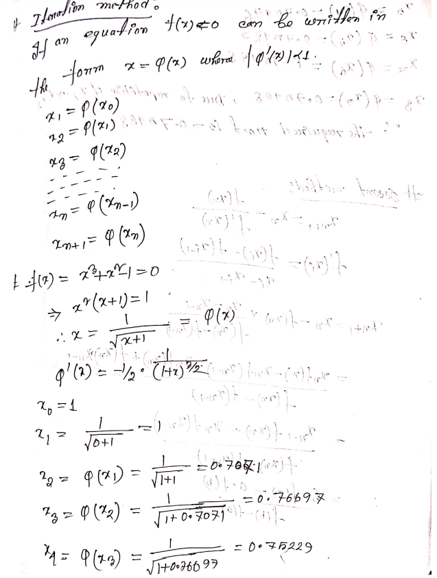
iretative method*
gauss-seidel method*
gauss-jordan*
taxonomoy of error*
shifting operator basic
Errors:
Error, in applied mathematics, the difference between a true value and an estimate, or approximation, of that value .
Taxonomy of error:
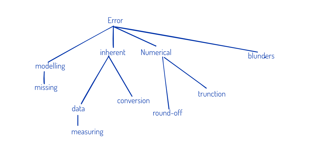
*truncation
Absolute Error
Absolute error is the difference between measured and the actual value of a quantity.
Keyword: measured value - actual value
If x is the actual value of a quantity and x0 is the measured value of the quantity, then the absolute error value can be calculated using the formula
Δx = |x0-x|.
Here, Δx is called an absolute error.
For example, 24.13 is the actual value of a quantity and 25.09 is the measure or inferred value, then the absolute error will be: Absolute Error = |25.09 – 24.13| = 0.86
Relative Error
The relative error is defined as the ratio of the absolute error of the measurement to the actual measurement.
Keyword: absolute error/actual error
If x is the actual value of a quantity, x0 is the measured value of the quantity and Δx is the absolute error, then the relative error can be measured using the below formula.
Relative error = (x0-x)/x = (Δx)/x
Rounding Error
Rounding error is the difference between a rounded-off numerical value and the actual value.
As an example of rounding error, consider the speed of light in a vacuum. The official value is 299,792,458 meters per second. In scientific (power-of-10) notation, that quantity is expressed as 2.99792458 x 10⁸. Rounding it to three decimal places yields 2.998 x 10⁸. The rounding error is the difference between the actual value and the rounded value, in this case (2.998 - 2.99792458) x 108, which works out to 0.00007542 x 10⁸ . Expressed in the correct scientific notation format, that value is 7.542 x 10³.
Rounding error = |rounded-off numerical value - actual value|
Percentage of Error
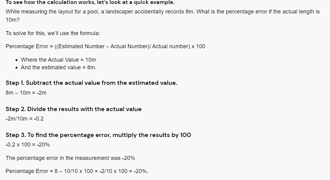
(Take absolute value)
Summary:
- Absolute Error = |Experimental Measurement – Actual Measurement|
- Relative Error= Absolute Error/Actual Measurement
- Percentage Error = Decimal Form of Relative Error x 100.
Truncation error
A truncation error is the difference between an actual and a truncated, or cut-off, value.
A truncated quantity is represented by a numeral with a fixed number of allowed digits, with any excess digits chopped off -- hence, the expression truncated
Example:
Consider the speed of light in a vacuum. The official value is 299,792,458 meters per second (m/s). In scientific (power-of-10) notation, it is expressed as 2.99792458 x 10⁸ m/s. But truncating it to only two decimal places yields 2.99 x 10⁸ m/s.
Since the truncation error is the difference between the actual value and the truncated value, in this case, it comes to the following:
2.99792458 x 10⁸ - 2.99 x 108 = 0.00792458 x 10⁸ m/s
Chopping Error:
- a type of round-off error
- truncated or chopping the last digit or last digit of a rounding value
(IT”S NOT A TURNCATION ERROR)
Transcendental Functions
The transcendental function can be defined as a function that is not algebraic and cannot be expressed in terms of a finite sequence of algebraic operations such as sin x.
Keyword: function which output is an infinite sequence
Transcendental equation
A transcendental equation is an equation into which transcendental functions (such as exponential, logarithmic, trigonometric, or inverse trigonometric) of one of the variables (s) have been solved for.
A transcendental equation is an equation over the real (or complex) numbers that is not algebraic, that is, if at least one of its sides describes a transcendental function.[1]
Keyword: the equation which contains transcendental function
Characteristics (NOT SURE)
- non-algebraic
- infinite
- contains transcendental functions
(learn more : https://www.britannica.com/science/transcendental-function)
(If you are more interested about Errors, learn from : https://graphics.stanford.edu/courses/cs205a-13-fall/assets/notes/chapter1.pdf . Anyways, I haven’t read the PDF yet. All of them are collected from different articles.)
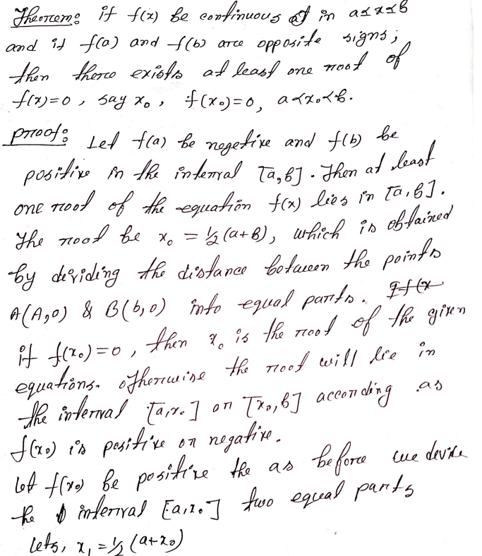
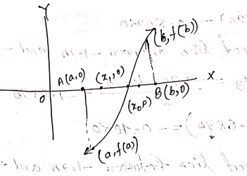
Bisection Method
The bisection method is an approximation method to find the roots of the given equation by repeatedly dividing the interval. This method will divide the interval until the resulting interval is found, which is extremely small.
More:
- used to find the roots of a polynomial equation
- based on intermediate theorem on continuous function
- work by narrowing the gap between positive and negative interval until closes in on the correct answer
Theory & Proof: (From Rupa)
Iterative Method
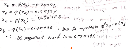
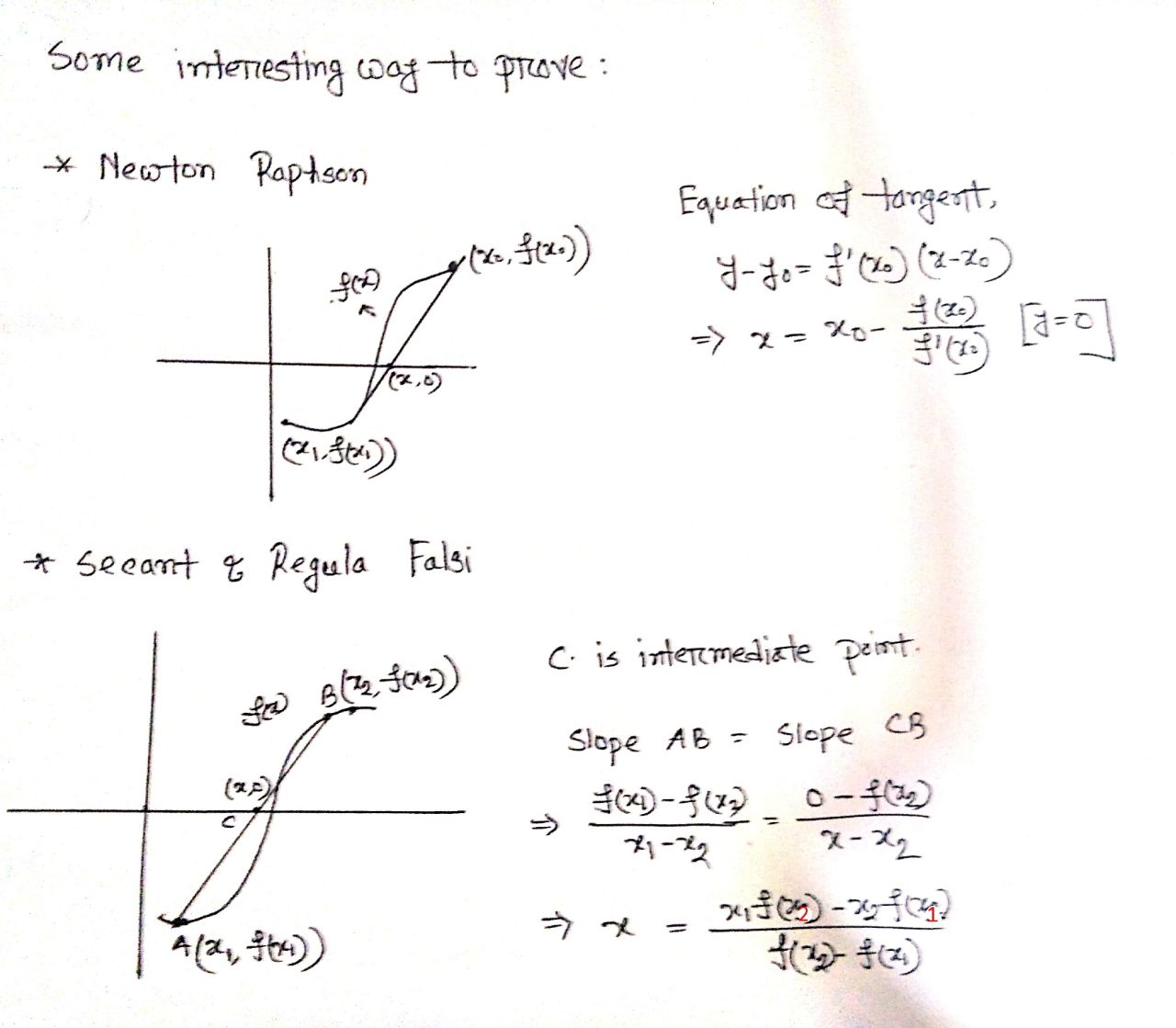
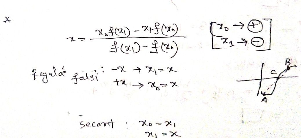
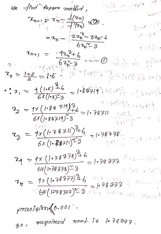
Newton Rapson Method
Theory & Proof : (from Rupa)

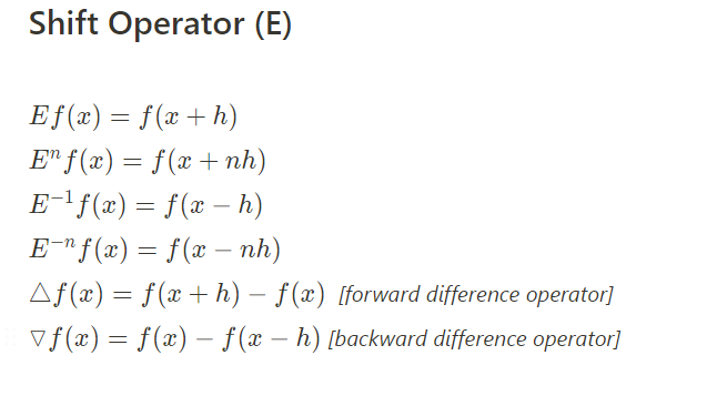
Shifting Operator
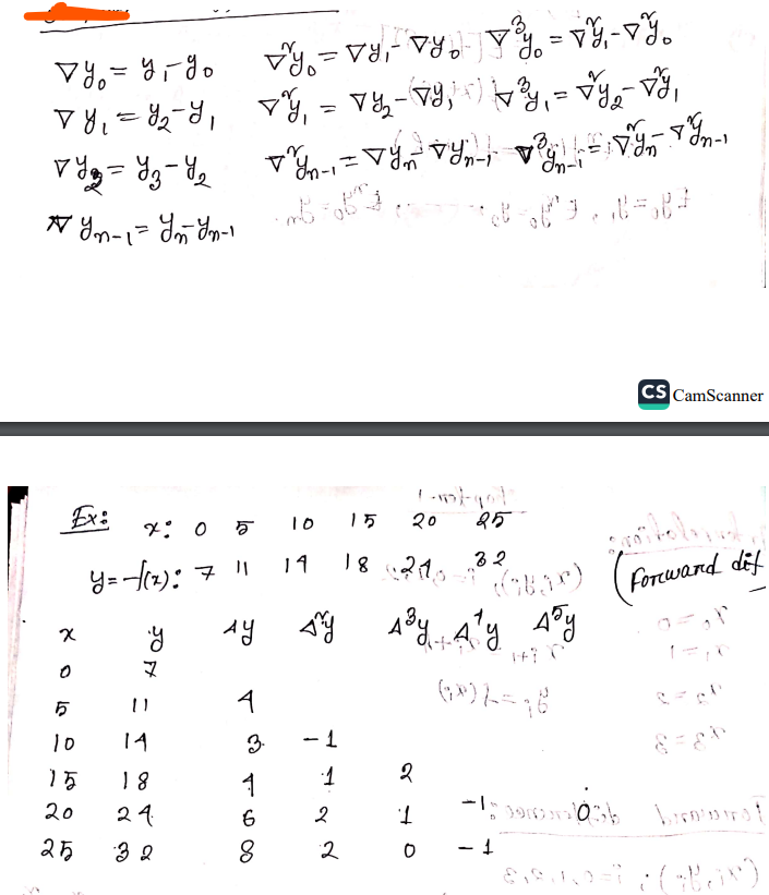
Forward Difference Table
Construct Forward Difference Table : (from Rupa)
Interpolation
In short, interpolation is a process of determining the unknown values that lie in between the known data points
x = 3 5 7 9 11
y= 2 6 8 12 13
The difference between and is equal. 2 for this example.
if,
x= 3.5 (at starting ) → we will use Newton Forward Interpolation
x= 5.1 - 7.9 → we will use Central Difference Interpolation (Out of syllabus)
x=9.5 (at end) → we will use Newton Backward Interpolation
Newton Forward Interpolation
Proof (from Rupa):
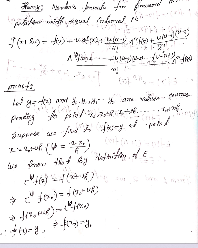
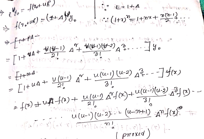
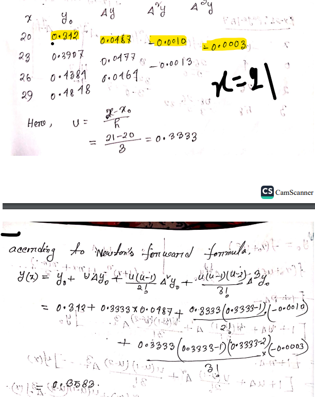
Math : (from Rupa)
Procedure:
- Create a difference table
- Use the formula and calculate
- h = difference b/w two contiguous x
- f(a), f^2(a), …. → upper value (1st row)
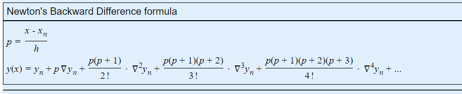
Newton Backward Interpolation
less important
- starting from below
- ‘+’ sign instead of ‘-’
(start taking the value of y from bottom → lower value)
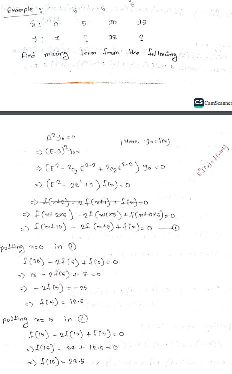
Missing Term in Interpolation
(YT: https://www.youtube.com/watch?v=P7fvPqdNOjM&ab_channel=B.K.TUTORIALS)
From Mishu:
Newton Divided Difference
What is Curve Fitting ?
(mark 4)
Curve fitting is the process of constructing a curve, or mathematical function, that has the best fit to a series of data points
Advantages:
- Simplicity: It is very easy to explain and to understand
- Applicability: There are hardly any applications where least squares doesn’t make sense
- Theoretical Underpinning: It is the maximum-likelihood solution and, if the Gauss-Markov conditions apply, the best linear unbiased estimator
Disadvantages/Drawbacks:***
- Sensitivity to outliers
- Test statistics might be unreliable when the data is not normally distributed (but with many datapoints that problem gets mitigated)
- Tendency to overfit data (LASSO or Ridge Regression might be advantageous)
- It can be quite sensitive to the choice of starting values.
- It is not readily applicable to censored data
Numerical Integration
Numerical Integration is a process of evaluating or obtaining a definite integral from a set of numerical values of the integrand f(x).
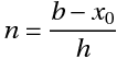
n = stripe, (generally, it’s 6. why 6 ? ⇒ because 6 is divisible by 2 and 3 ? Why 2 & 3 ? Check below ?)
Trapezoidal Rule
Applicable for any no. interval.
Simpson one-third rule
Applicable for only even intervals.
Simpson three-by-eight rule
Applicable for only multiple of 3 intervals.
WHY 6 ? ⇒ Because 6 is an even multiple of 3. And it’s the minimum which fill-up both conditions.
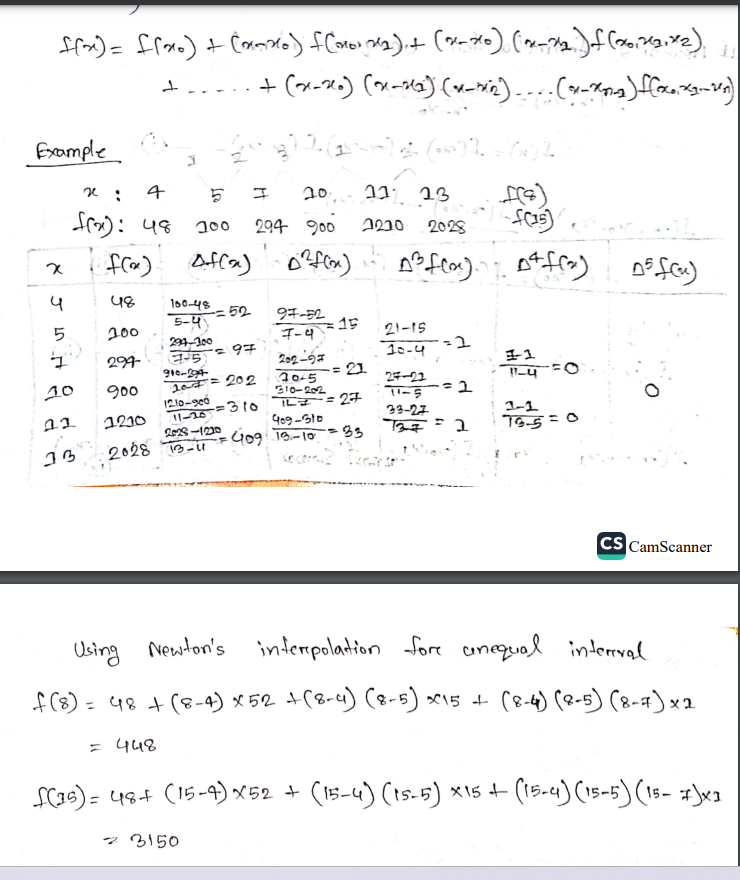
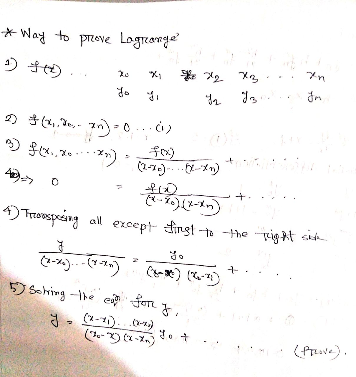
Lagrange Interpolation
The Lagrange interpolation formula is a way to find a polynomial which takes on certain values at arbitrary points
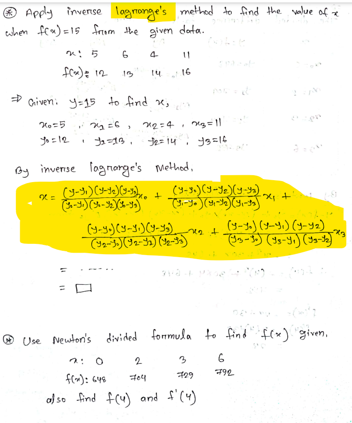
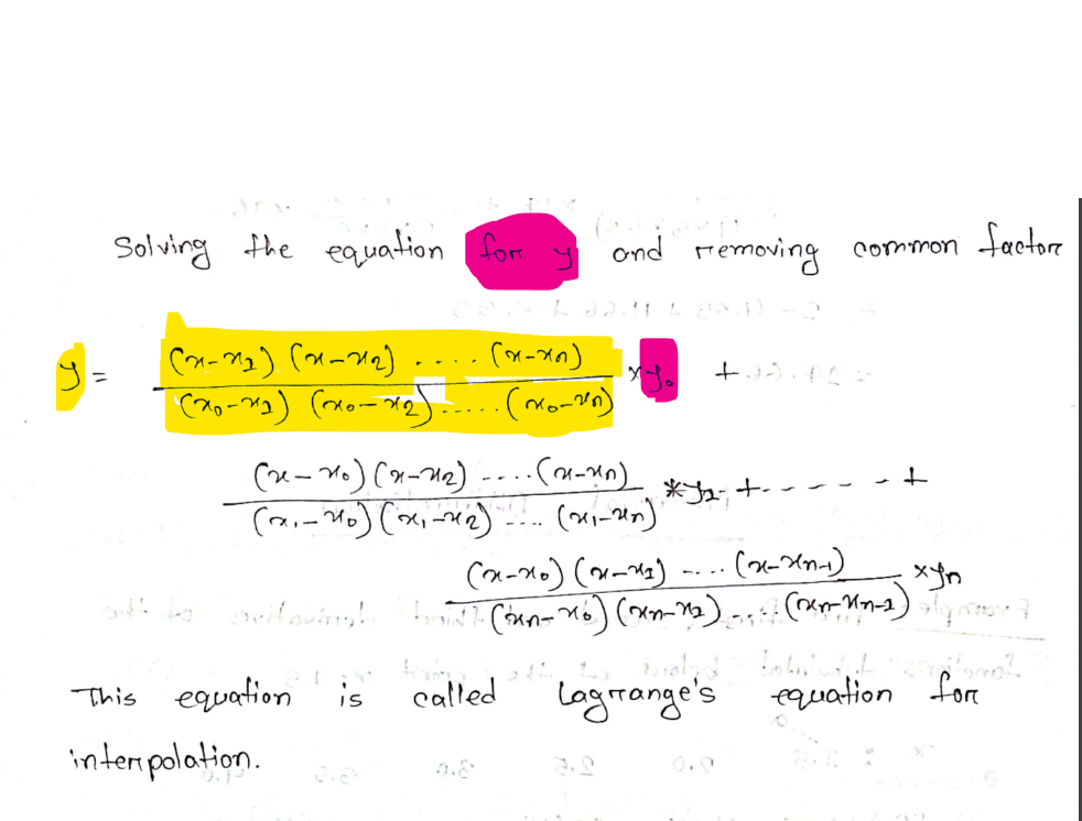
Approaches to Prove Lagrange:
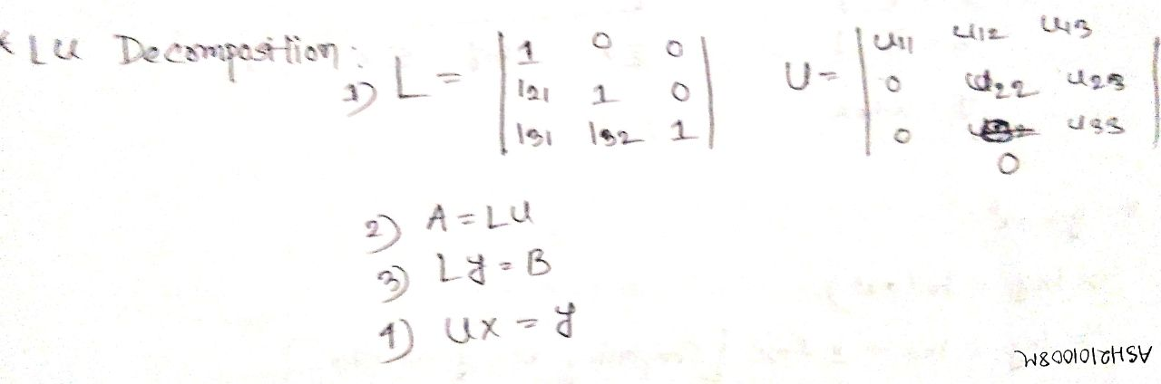
LU Decomposition Factorization
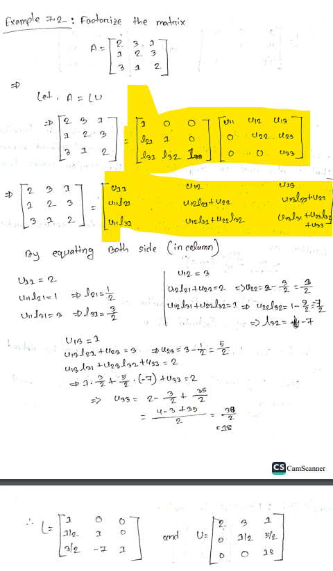
To solve the Equation using LU Decomposition:
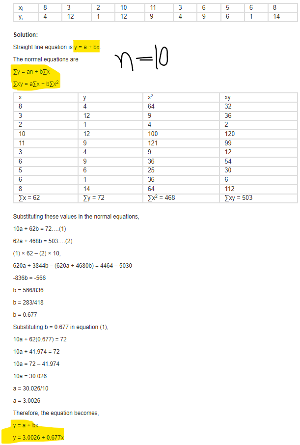
Least Square Method
The least square method is the process of finding the best-fitting curve or line of best fit for a set of data points by reducing the sum of the squares of the points from the curve.
The equation of least square line is given by Y = a + bX
Normal equation for ‘a’:
∑Y = na + b∑X
Normal equation for ‘b’:
∑XY = a∑X + b∑X2
Question 1.: Find a straight line that fits the following data
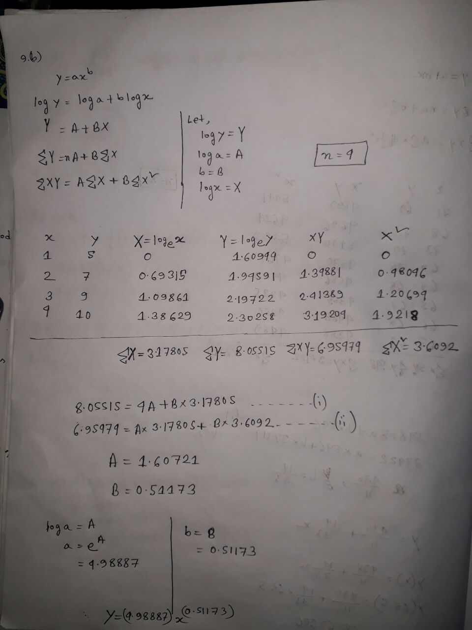
Question 2 :
- y=something-something convert it to y=a+bx, and find new A, X, Y
- Create table
- Use those two formula and get the value of A,b … convert A to a.
From Fayaz:
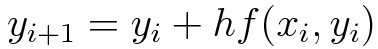
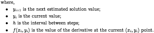
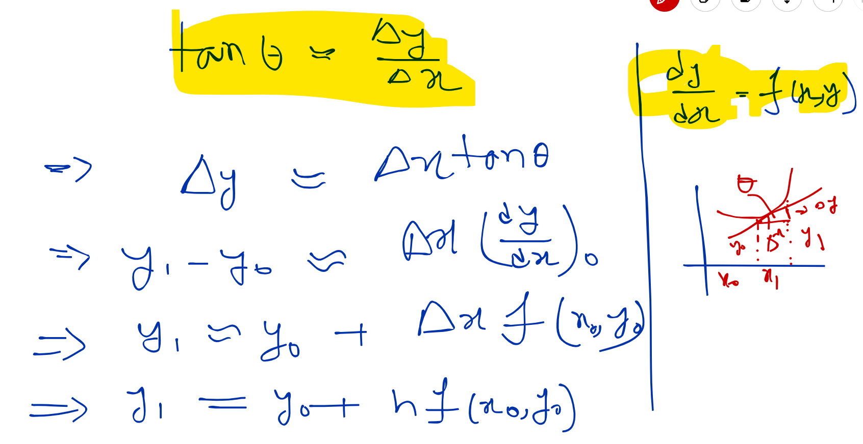
Euler Method:
(https://www.youtube.com/watch?v=u5ggAyOOTUw&t=19s)
The Euler’s method is a first-order numerical procedure for solving ordinary differential equations (ODE) with a given initial value.
Euler proof (Approach) :
Modified Euler Method:
(https://www.youtube.com/watch?v=xLGDGeFZTnQ)
Instead of approximating f(x, y) by as in Euler’s method. In the Modified Euler Method: we have the iteration formula
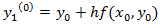
Take to solve it by one step.
Accuracy
Euler method has a truncation error. To solve this problem modified Euler method is introduced. How ? →
- It takes arithmetic average of an interval (Xi, Xi+1) instead of a point. bla bla bla….
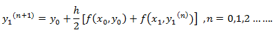
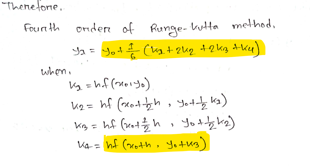
Range Kutta Method
(https://www.youtube.com/watch?v=fll1HdYy6vk&t=696s - 2nd Order)
(https://www.youtube.com/watch?v=JhI6cLRjKHY - 4th Order)
Runge–Kutta method is an effective and widely used method for solving the initial-value problems of differential equations. Runge–Kutta method can be used to construct high order accurate numerical method by functions' self without needing the high order derivatives of functions.
4th Order from Mishu:
Gauss Seidel Method
 https://byjus.com/maths/iterative-methods-gauss-seidel-and-jacobi/

Preferred Initial value, x1=x2=x3=0
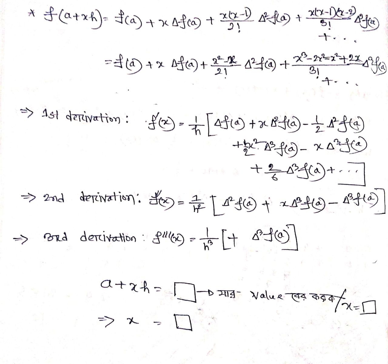
Numerical Differentiation:
- Create Forward Difference Table
- Use the formulae for 1st, 2nd and 3rd derivative
Different between Gauss Elimination Method & Gauss Jordan Method
In mathematics, the Gaussian elimination method is known as the row reduction algorithm for solving linear equations systems.
| Gauss Elimination Method | Gauss Jordan Method |
| upper triangular system | reduces to diagonal matrix |
| For large systems, Gauss Elimination Method is not preferred. | For large systems, Gauss Jordan Method is preferred to Gauss Elimination Method |
| It does not seem to be easier | It seems to be easier |
| it requires about 50 percent fewer operation than | requires about 50 percent more operations than Gauss elimination Method. |
EXTRA:
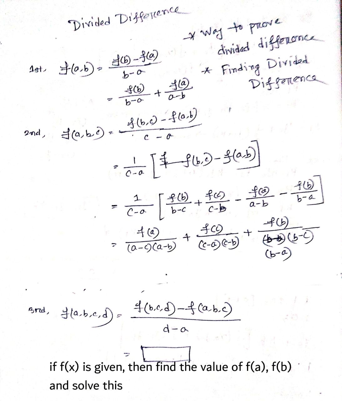
Divided Difference Proof Idea and finding nth Divided Difference
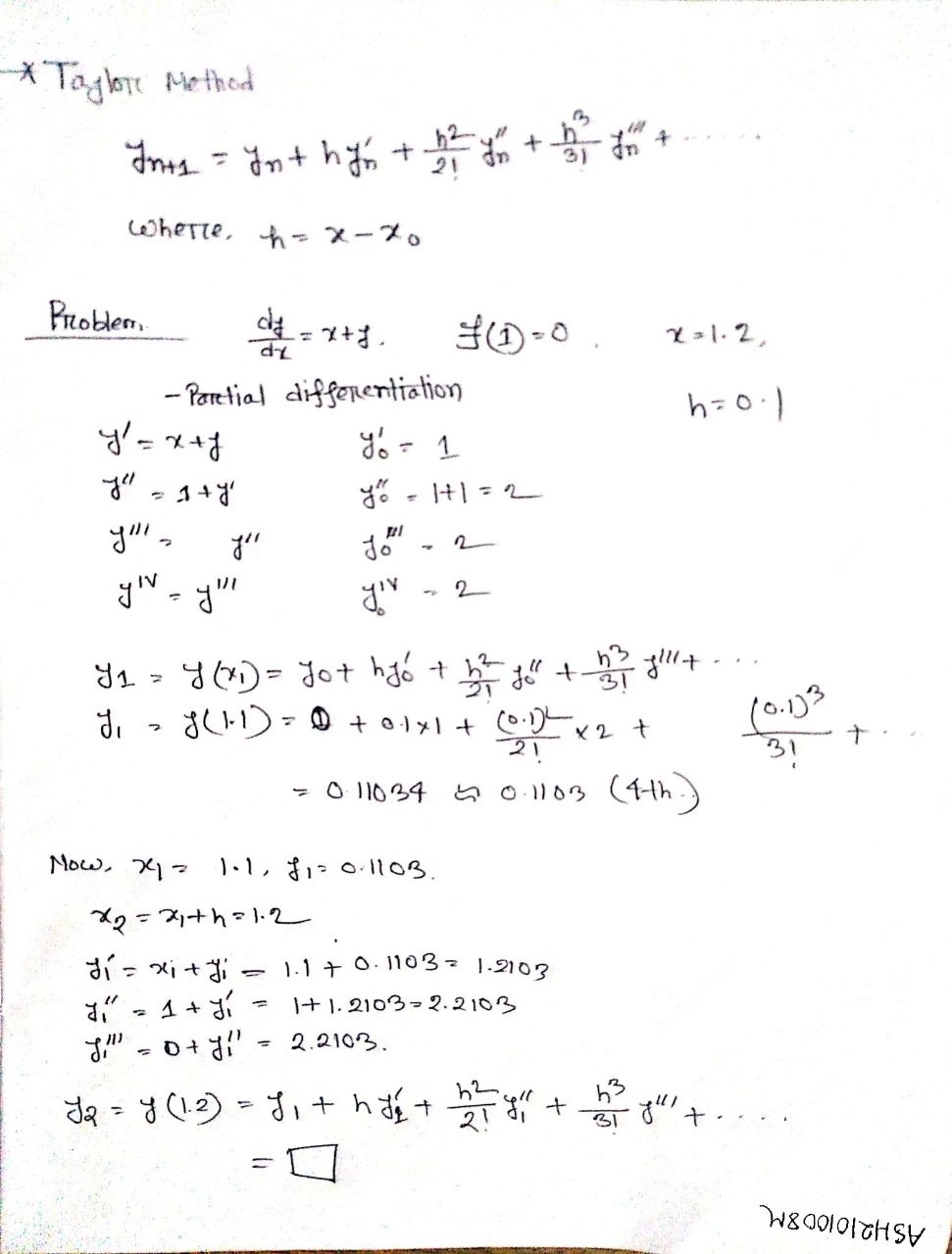
Taylor:
(https://www.youtube.com/watch?v=82IDoaiYU0c&ab_channel=MKSTUTORIALSbyManojSir)